An incumbent president running for re-election reaps both benefits and barriers. For one, they are a candidate that the American people are familiar with and normalized to. That being said, the American people also have four years of work to analyze and interpret. The condition of the United States is put on the sitting Commander-in-Chief who is already in the position to lead the economy, culture, and social circumstances of their country. In the past decade, we’ve seen Former President Barack Obama benefit in his re-election campaign against Mitt Romney, having been in a post-Hurricane Sandy relief era and reviving the economy after a significant bump during his mid-terms. On the other end, we saw Former President Donald Trump face the repercussions of controversial foreign relations, poor COVID-19 relief, and high unemployment in 2020. With this in mind, my second blog post will focus on different independent variables that can be used to predict the outcome of the 2024 election. Specifically, I will use economic variables to analyze their predictive abilities in elections between 1948 and 2020, in order to see the variable(s) best suited to predict the election in November.
Growth Domestic Product
First, I will look at the relationship between GDP and the incumbent party’s vote share. Gross Domestic Product (GDP) measures the total value of all goods and services produced within a country. It is a crucial indicator for assessing the overall strength of the economy, showing whether it is expanding or contracting.
d_inc_econ |>
  ggplot(aes(x = GDP_growth_quarterly, y = pv2p, label = year)) +
  geom_text() +
  geom_hline(yintercept = 50, lty = 2) +
  geom_vline(xintercept = 0.01, lty = 2) +
  labs(title = "Relationship Between GDP Growth and Incumbent Voter Share",
       subtitle = "1948-2020",
       x = "Second Quarter GDP Growth (%)",
       y = "Incumbent Party's National Popular Vote Share") +
  my_blog_theme()
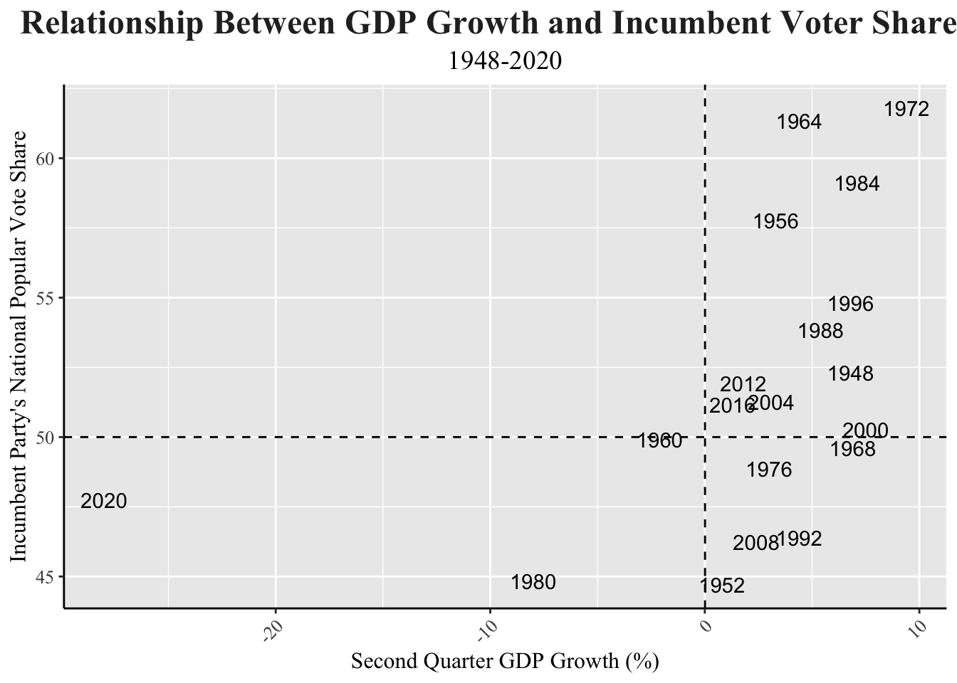
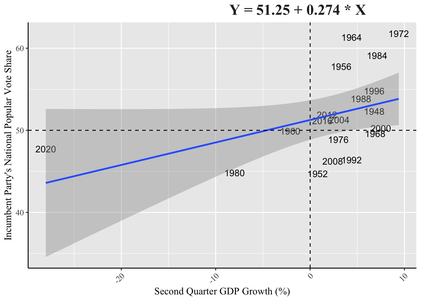
It’s clear that 2020 is a significant outlier in this plot, having an extreme decrease in GDP growth, due to the pandemic. The dashed lines organize the information to showcase election years where there was growth versus loss, as well as popular vote victory versus losses for the incumbent party. A majority of election years where there was GDP growth also presented popular vote victories. The plot below better exemplifies this trend with a regression line drawn to show the positive correlation between GDP growth and vote share.
# Can add bivariate regression lines to our scatterplots.

d_inc_econ |>
  ggplot(aes(x = GDP_growth_quarterly, y = pv2p, label = year)) +
  geom_text() +
  geom_smooth(method = "lm", formula = y ~ x) +
  geom_hline(yintercept = 50, lty = 2) +
  geom_vline(xintercept = 0.01, lty = 2) +
  labs(x = "Second Quarter GDP Growth (%)",
       y = "Incumbent Party's National Popular Vote Share",
       title = "Y = 51.25 + 0.274 * X") +
  my_blog_theme() +
  theme(plot.title = element_text(size = 18))
## Warning: The following aesthetics were dropped during statistical transformation: label
## ℹ This can happen when ggplot fails to infer the correct grouping structure in
##   the data.
## ℹ Did you forget to specify a `group` aesthetic or to convert a numerical
##   variable into a factor?
summary(reg_econ)$r.squared
## [1] 0.1880919
I ran the same model twice, to see the impact of including 2020 despite it being an outlier. The first data set has a R squared value of 0.1881, while the second data set, which excludes the 2020 election year, has a R squared value of 0.3248. The R squared value helps identify how strongly the independent variable can be predicted by the dependent variable. In this case, the regression seeks to find out the relationship between GDP growth in the second quarter and the incumbent party’s popular vote share. The Y variable (vote share) can be better predicted based on the X variable (GDP growth) when 2020 is excluded. However, for the rest of the blog I will continue to use data that includes the 2020 election year, due to its proximity in relevance in this year’s election with the impact of issues like COVID-19, race relations, and economic discourse still relevant. While the predictions may have a lower R-squared value in aligning previous elections, the inclusion of 2020 will be a better predictor for the 2024 election.
Consumer Price Index
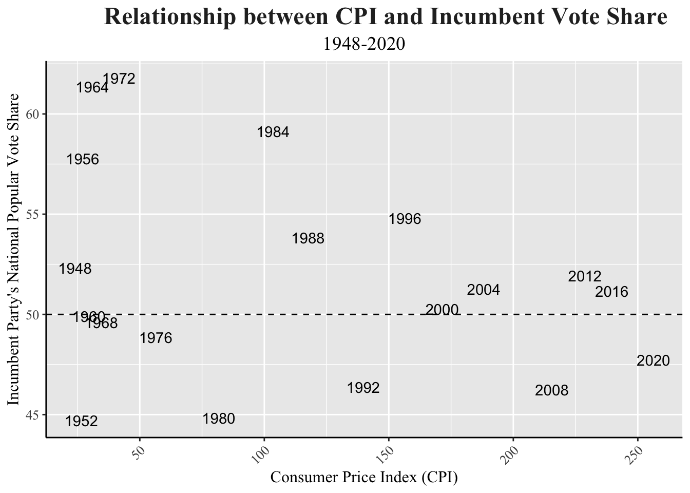
The Consumer Price Index (CPI) is a measure that examines the average change over time in the prices paid by urban consumers for goods and services. It’s a key indicator of inflation and reflects changes in the cost of living. In the context of elections, the CPI can significantly impact the incumbent party’s chances of re-election. When inflation is high, as indicated by a rising CPI, the cost of living increases, which leads to economic dissatisfactio as people must use more of their income on basic needs. This dissatisfaction often translates into political discontent, as voters may blame the incumbent administration for not effectively managing the economy. Conversely, if the CPI shows stable or low inflation, it suggests that the cost of living is relatively manageable, which can uplift the incumbent party’s vote share in re-election.
### Relationship between CPI and vote share

# Create scatter plot to visualize relationship between CPI and incumbent vote share.
d_inc_econ |>
  ggplot(aes(x = CPI, y = pv2p, label = year)) +
  geom_text() +
  geom_hline(yintercept = 50, lty = 2) +
  labs(title = "Relationship between CPI and Incumbent Vote Share",
       subtitle = "1948-2020",
       x = "Consumer Price Index (CPI)",
       y = "Incumbent Party's National Popular Vote Share") +
  my_blog_theme()
d_inc_econ |>
ggplot(aes(x = CPI, y = pv2p, label = year)) +
geom_text() +
geom_smooth(method = "lm", formula = y ~ x) +
geom_hline(yintercept = 50, lty = 2) +
labs(title = "Relationship between CPI and Incumbent Vote Share",
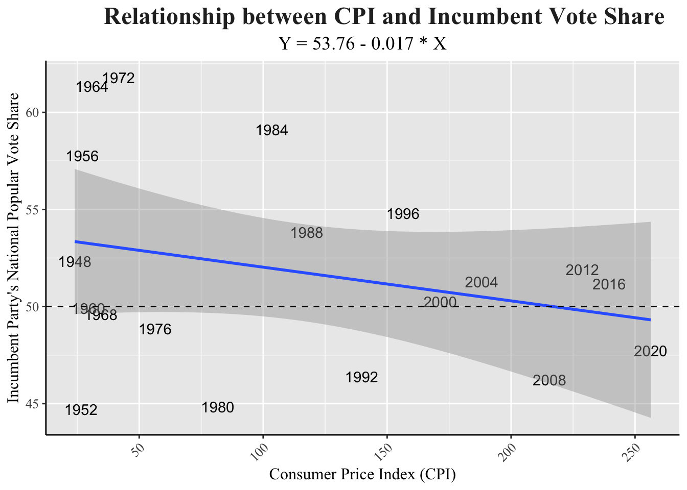
subtitle = "Y = 53.76 - 0.017 * X",
x = "Consumer Price Index (CPI)",
y = "Incumbent Party's National Popular Vote Share") +
my_blog_theme() +
theme(plot.title = element_text(size = 18))
## Warning: The following aesthetics were dropped during statistical transformation: label
## ℹ This can happen when ggplot fails to infer the correct grouping structure in
##   the data.
## ℹ Did you forget to specify a `group` aesthetic or to convert a numerical
##   variable into a factor?
# Compute correlations between CPI and incumbent vote 2-party vote share.
cor(d_inc_econ$CPI,
    d_inc_econ$pv2p)
## [1] -0.2762669
cor(d_inc_econ_2$CPI,
    d_inc_econ_2$pv2p)
## [1] -0.2218343
# Fit bivariate OLS.
reg_cpi <- lm(pv2p ~ CPI,
               data = d_inc_econ)
reg_cpi |> summary()
##
## Call:
## lm(formula = pv2p ~ CPI, data = d_inc_econ)
##
## Residuals:
##     Min      1Q  Median      3Q     Max
## -8.5915 -3.6807 -0.5288  2.9385  8.7491
##
## Coefficients:
##             Estimate Std. Error t value Pr(>|t|)
## (Intercept) 53.76136    2.04701  26.263 3.35e-15 ***
## CPI         -0.01734    0.01463  -1.185    0.252
## ---
## Signif. codes:  0 '***' 0.001 '**' 0.01 '*' 0.05 '.' 0.1 ' ' 1
##
## Residual standard error: 5.156 on 17 degrees of freedom
## Multiple R-squared:  0.07632,	Adjusted R-squared:  0.02199
## F-statistic: 1.405 on 1 and 17 DF,  p-value: 0.2522
reg_cpi_2 <- lm(pv2p ~ CPI,
                         data = d_inc_econ_2)
reg_cpi_2 |> summary()
##
## Call:
## lm(formula = pv2p ~ CPI, data = d_inc_econ_2)
##
## Residuals:
##     Min      1Q  Median      3Q     Max
## -8.4949 -3.7923 -0.1371  3.1621  8.8106
##
## Coefficients:
##             Estimate Std. Error t value Pr(>|t|)
## (Intercept) 53.60353    2.15372   24.89 3.21e-14 ***
## CPI         -0.01503    0.01651   -0.91    0.376
## ---
## Signif. codes:  0 '***' 0.001 '**' 0.01 '*' 0.05 '.' 0.1 ' ' 1
##
## Residual standard error: 5.296 on 16 degrees of freedom
## Multiple R-squared:  0.04921,	Adjusted R-squared:  -0.01021
## F-statistic: 0.8281 on 1 and 16 DF,  p-value: 0.3763
As CPI increased, incumbent party vote share also decreases, which aligns with my original hypothesis, as voter satisfaction decreases with increased cost of living. 2020 does not stand as an outlier, despite the pandemic’s impact. The R-squared value for this regression is 0.049.
Unemployment
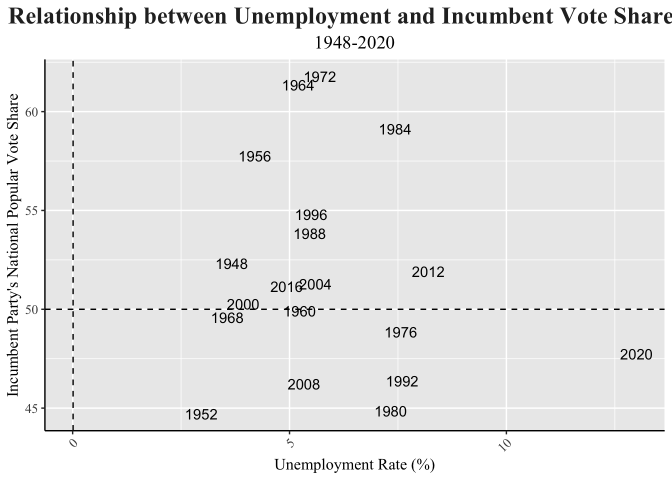
The unemployment rate measures the percentage of people actively seeking work but unable to find jobs. A high unemployment rate may lead voters to favor the opposite party, if they are promising better job creation and economic policies.
### Relationship between unemployment and vote share

# Create scatter plot to visualize relationship between CPI and incumbent vote share.
d_inc_econ |>
  ggplot(aes(x = unemployment, y = pv2p, label = year)) +
  geom_text() +
  geom_hline(yintercept = 50, lty = 2) +
  geom_vline(xintercept = 0.01, lty = 2) +
  labs(title = "Relationship between Unemployment and Incumbent Vote Share",
       subtitle = "1948-2020",
       x = "Unemployment Rate (%)",
       y = "Incumbent Party's National Popular Vote Share") +
  my_blog_theme()
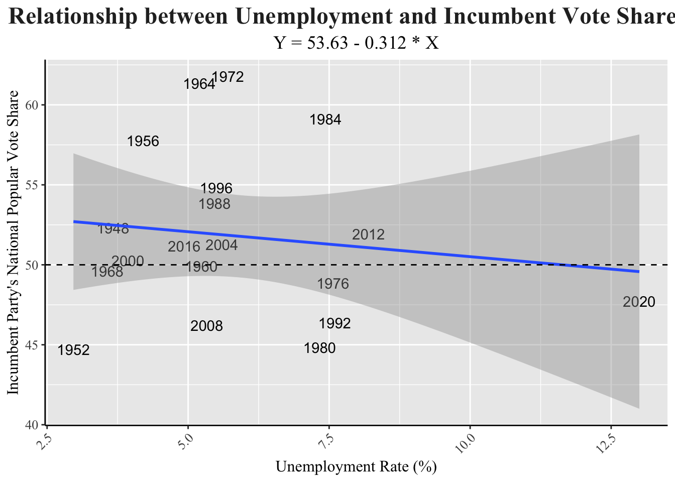
d_inc_econ |>
  ggplot(aes(x = unemployment, y = pv2p, label = year)) +
  geom_text() +
  geom_smooth(method = "lm", formula = y ~ x) +
  geom_hline(yintercept = 50, lty = 2) +
  labs(title = "Relationship between Unemployment and Incumbent Vote Share",
       subtitle = "Y = 53.63 - 0.312 * X",
       x = "Unemployment Rate (%)",
       y = "Incumbent Party's National Popular Vote Share") +
  my_blog_theme() +
  theme(plot.title = element_text(size = 18))
## Warning: The following aesthetics were dropped during statistical transformation: label
## ℹ This can happen when ggplot fails to infer the correct grouping structure in
##   the data.
## ℹ Did you forget to specify a `group` aesthetic or to convert a numerical
##   variable into a factor?
# Compute correlations between CPI and incumbent vote 2-party vote share.
cor(d_inc_econ$unemployment,
    d_inc_econ$pv2p)
## [1] -0.1368118
cor(d_inc_econ_2$unemployment,
    d_inc_econ_2$pv2p)
## [1] 0.006522146
# Fit bivariate OLS.
reg_unemp <- lm(pv2p ~ unemployment,
               data = d_inc_econ)
reg_unemp |> summary()
##
## Call:
## lm(formula = pv2p ~ unemployment, data = d_inc_econ)
##
## Residuals:
##     Min      1Q  Median      3Q     Max
## -7.9906 -2.6616 -0.9256  2.4016  9.9399
##
## Coefficients:
##              Estimate Std. Error t value Pr(>|t|)
## (Intercept)   53.6260     3.4614  15.493 1.85e-11 ***
## unemployment  -0.3117     0.5475  -0.569    0.577
## ---
## Signif. codes:  0 '***' 0.001 '**' 0.01 '*' 0.05 '.' 0.1 ' ' 1
##
## Residual standard error: 5.314 on 17 degrees of freedom
## Multiple R-squared:  0.01872,	Adjusted R-squared:  -0.03901
## F-statistic: 0.3243 on 1 and 17 DF,  p-value: 0.5765
reg_unemp_2 <- lm(pv2p ~ unemployment,
                         data = d_inc_econ_2)
reg_unemp_2 |> summary()
##
## Call:
## lm(formula = pv2p ~ unemployment, data = d_inc_econ_2)
##
## Residuals:
##     Min      1Q  Median      3Q     Max
## -7.2394 -2.9835 -0.7848  2.5555  9.7788
##
## Coefficients:
##              Estimate Std. Error t value Pr(>|t|)
## (Intercept)  51.88452    4.84160  10.716 1.04e-08 ***
## unemployment  0.02205    0.84527   0.026     0.98
## ---
## Signif. codes:  0 '***' 0.001 '**' 0.01 '*' 0.05 '.' 0.1 ' ' 1
##
## Residual standard error: 5.431 on 16 degrees of freedom
## Multiple R-squared:  4.254e-05,	Adjusted R-squared:  -0.06245
## F-statistic: 0.0006806 on 1 and 16 DF,  p-value: 0.9795
As the unemployment rate increases, the incumbent party has a lower vote share. The R-value on this is extremely low though, so it would definitely not be a good predictor for this election.
Predicting 20204 Election Results
With the GDP, CPI, and unemployment regressions all run, we can now use previous election trends to see the outcomes on vote share of the incumbent party for the 2024 election. The GDP data predicts that the Democratic party will receive 51.6% of the vote share. CPI predicts 49.3%, and unemployment predicts 52.1%.
Best Predictor
GDP growth in the second quarter is the best predictor for the incumbent party’s vote share in the 2024 election, since it has the highest R-squared value out of the three variables investigated in this blog. Using the variable, the Democratic party will win this election. However, the r-squared value is 0.3, so it is still not a great predictor. In a further investigation, I would continue to look at other variables and potentially run a multi-variable regression to better predict variability.
Sources
https://www.bls.gov/cpi/factsheets/averages-and-individual-experiences-differ.htm
https://www.pewresearch.org/politics/2021/06/30/behind-bidens-2020-victory/